8 Statistical Modeling and Supervised Machine Learning
Abstract. This chapter introduces the reader to the world of supervised machine learning. It starts by outlining how classical statistical techniques such as regression models can be used for prediction. It then provides an overview of frequently-used techniques from Naïve Bayes classifiers to neural networks.
Keywords. supervised machine learning
Objectives: - Understand the principles of supervised machine learning - Be able to run a predictive model - Be able to evaluate the performance of a predictive model
In this chapter, we introduce the basic concepts and ideas behind machine learning. We will outline how machine learning relates to traditional statistical approaches that you already might know (and as you will see, there is a lot of overlap), present different types of models, and discuss how to validate them. Later in this book (Section 11.4), we will specifically apply the knowledge you gain from this chapter to the analysis of textual data, arguably one of the most interesting tasks in the computational analysis of communication.
In this chapter, we focus on supervised machine learning (SML) – a form of machine learning, where we aim to predict a variable that, for at least a part of our data, is known. SML is usually applied to classification and regression problems. To illustrate the idea, imagine that you are interested in predicting gender, based on Twitter biographies. You determine the gender for some of the biographies yourself and hand these examples over to the computer. The computer “learns” this classification from your examples, and can then be used to predict the gender for other Twitter biographies for which you do not know the gender.
In unsupervised machine learning (UML), in contrast, you do not have such examples. Therefore, UML is usually applied to clustering and associations problems. We have discussed some of these techniques in Section 7.3, in particular cluster analysis and principal component analysis (PCA). Later, in Section 11.5, we will discuss topic modeling, an unsupervised method to extract so-called topics from textual data.
Even though both approaches can be combined (for instance, one could first reduce the amount of data using PCA or SVD, and then predict some outcome), they can be seen as fundamentally different, from both theoretical and conceptual points of view. Unsupervised machine learning is a bottom-up approach and corresponds to an inductive reasoning: you do not have a hypothesis of, for instance, which topics are present in a corpus of text; you rather let the topics emerge from the data. Supervised machine learning, in contrast, is a top-down approach and can be seen as more deductive: you define a priori which topics to predict.
8.1 Statistical Modeling and Prediction
Machine learning, many people joke, is nothing other than a fancy name for statistics. And, in fact, there is some truth to this: if you say “logistic regression”, this will sound familiar to both statisticians and machine learning practitioners. Hence, it does not make much sense to distinguish between statistics on the one hand and machine learning on the other hand. Still, there are some differences between traditional statistical approaches that you may have learned about in your statistics classes and the machine learning approach, even if some of the same mathematical tools are used. One may say that the focus is a different one, and the objective we want to achieve may differ.
Let us illustrate this with an example. media.csv1 contains a few columns from survey data on how many days per week respondents turn to different media types (radio, newspaper, tv and Internet) in order to follow the news2. It also contains their age (in years), their gender (coded as female = 0, male = 1), and their education (on a 5-point scale).
A straightforward question to ask is how far the sociodemographic characteristics of the respondents explain their media use. Social scientists would typically approach this question by running a regression analysis. Such an analysis tells us how some independent variables \(x_1, x_2, \ldots, x_n\) can explain \(y\). In an ordinary least square regression (OLS), we would estimate \(y=\beta_0 + \beta_1 x_1 + \beta_2 x_2 + \ldots + \beta_n x_n\).
In a typical social-science paper, we would then interpret the coefficients that we estimated, and say something like: when \(x_1\) increases by one unit, \(y\) increases by \(\beta_1\). We sometimes call this “the effect of \(x_1\) on \(y\)” (even though, of course, it depends on the study design whether the relationship can really be interpreted as a causal effect). Additionally, we might look at the explained variance \(R^2\), to assess how well the model fits our data. In Example 8.1 we use this regression approach to model the relationship of age and gender over the number of days per week a person reads a newspaper. We fit the linear model using the stats function lm in R and the statsmodels function ols (imported from the module statsmodels.formula.api) in Python.
Most traditional social-scientific analyses stop after reporting and interpreting the coefficients of age (\(\beta = 0.0676\)) and gender (\(\beta = -0.0896\)), as well as their standard errors, confidence intervals, p-values, and the total explained variance (19%). But we can go a step further. Given that we have already estimated our regression equation, why not use it to do some prediction?
We have just estimated that
By just filling in the values for a 20 year old man, or a 40 year old woman, we can easily calculate the expected number of days such a person reads the newspaper per week, even if no such person exists in the original dataset.
We learn that
This was easy to do by hand, but of course, we could do this automatically for a large and essentially unlimited number of cases. This could be as simple as shown in Example 8.2.
In doing so, we shift our attention from the interpretation of coefficients to the prediction of the dependent variable for new, unknown cases. We do not care about the actual values of the coefficients, we just need them for our prediction. In fact, in many machine learning models, we will have so many of them that we do not even bother to report them.
As you see, this implies that we proceed in two steps: first, we use some data to estimate our model. Second, we use that model to make predictions.
We used an OLS regression for our first example, because it is very straightforward to interpret and most of our readers will be familiar with it. However, a model can take the form of any function, as long as it takes some characteristics (or “features”) of the cases (in this case, people) as input and returns a prediction.
Using such a simple OLS regression approach for prediction, as we did in our example, can come with a couple of problems, though. One problem is that in some cases, such predictions do not make much sense. For instance, even though we know that the output should be something between 0 and 7 (as that is the number of days in a week), our model will happily predict that once a man reaches the age of 105 (rare, but not impossible), he will read a newspaper on 7.185 out of 7 days. Similarly, a one year old girl will even have a negative amount of newspaper reading. A second problem relates to the models’ inherent assumptions. For instance, in our example it is quite an assumption to make that the relationships between these variables are linear –- we will therefore discuss multiple models that do not make such assumptions later in this chapter. And, finally, in many cases, we are actually not interested in getting an accurate prediction of a continuous number (a regression task), but rather in predicting a category. We may want to predict whether a tweet goes viral or not, whether a user comment is likely to contain offensive language or not, whether an article is more likely to be about politics, sports, economy, or lifestyle. In machine learning terms, these tasks are known as classification.
In the next section, we will outline key terms and concepts in machine learning. After that, we will discuss specific models that you can use for different use applications.
8.2 Concepts and Principles
The goal of Supervised Machine Learning can be summarized in one sentence: estimate a model based on some data, and then use the model to predict the expected outcome for some new cases, for which we do not know the outcome yet. This is exactly what we have done in the introductory example in Section 8.1.
But when do we need it?
In short, in any scenario where the following two preconditions are fulfilled. First, we have a large dataset (say, \(100000\) headlines) for which we want to predict to which class they belong to (say, whether they are clickbait or not). Second, for a random subset of the data (say, \(2000\) of the headlines), we already know the class. For example because we have manually coded (“annotated”) them.
Before we start using SML, though, we first need to have a common terminology. At the risk of oversimplifying matters, Table 8.1 provides a rough guideline of how some typical machine learning terms translate to statistical terms that you may be familiar with.
| machine learning lingo | statistics lingo |
|---|---|
| feature | independent variable |
| label | dependent variable |
| labeled dataset | dataset with both independent and dependent variables |
| to train a model | to estimate |
| classifier (classification) | model to predict nominal outcomes |
| to annotate | to (manually) code (content analysis) |
Let us explain them more in detail by walking through a typical SML workflow.
Before we start, we need to get a labeled dataset. It may be given to us, or we may need to create it ourselves. For instance, often we can draw a random sample of our data and use techniques of manual content analysis (e.g., Riffe et al. 2019) to annotate (i.e., to manually code) the data. You can download an example for this process (annotating the topic of news articles) from dx.doi.org/10.6084/m9.figshare.7314896.v1 (Vermeer 2018).
It is hard to give a rule of thumb for how much labeled data you need. It depends heavily on the type of data you have (for instance, if it is a binary as opposed to a multi-class classification problem), and on how evenly distributed (class balance) they are (after all, having \(10000\) annotated headlines doesn’t help you if \(9990\) are not clickbait and only \(10\) are). These reservations notwithstanding, it is fair to say that typical sizes in our field are (very roughly) speaking often in the order of \(1000\) to \(10000\) when classifying longer texts (see Burscher et al. 2014), even though researchers studying less rich data sometimes annotate larger datasets (e.g., \(60000\) social media messages in Vermeer et al. 2019).
Once we have established that this labeled dataset is available and have ensured that it is of good quality, we randomly split it into two datasets: a training dataset and a test dataset.3 We will use the first one to train our model, and the second to test how well our model performs. Common ratios range from 50:50 to 80:20; and especially if the size of your labeled dataset is rather limited, you may want to have a slightly larger training dataset at the expense of a slightly smaller test dataset.
In Example 8.3, we prepare the dataset we already used in Section 8.1 for classification by creating a dichotomous variable (the label) and splitting it into a training and a test dataset. We use y_train to denote the training labels and X_train to denote the feature matrix of the training dataset; y_test and X_test is the corresponding test dataset. We set a so-called random-state seed to make sure that the random splitting will be the same when re-running the code. We can easily split these datasets using the rsample function initial_split in R and the sklearn function train_test_split in Python.
We now can train our classifier (i.e., estimate our model using the training dataset contained in the objects X_train and y_train). This can be as straightforward as estimating a logistic regression equation (we will discuss different classifiers in Section 8.3). It may be that we first need to create new independent variables, so-called features, a step known as feature engineering, for example by transforming existing variables, combining them, or by converting text to numerical word frequencies. Example 8.4 shows how easy it is to train a classifier using the Naïve Bayes algorithm with packages caret/naivebayes in R and sklearn in Python (this approach will be better explained in Section 8.3.1).
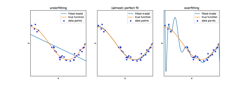
But before we can actually use this classifier to do some useful work, we need to test how capable it is to predict the correct labels, given a set of features. One might think that we could just feed it the same input data (i.e., the same features) again and see whether the predicted labels match the actual labels of the test dataset. In fact, we could do that. But this test would not be strict enough: after all, the classifier has been trained on exactly these data, and therefore one would expect it to perform pretty well. In particular, it may be that the classifier is very good in predicting its own training data, but fails at predicting other data, because it overgeneralizes some idiosyncrasy in the data, a phenomenon known as overfitting (see Figure 8.1).
Instead, we use the features of the test dataset (stored in the objects X_test and y_test) as input for our classifier, and evaluate how far the predicted labels match the actual labels. Remember: the classifier has at no point in time seen the actual labels. Therefore, we can in fact calculate how often the prediction is right.4
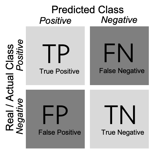
As shown in Example 8.5, we can create a confusion matrix (generated with caret function confusionMatrix in R and sklearn function confusion_matrix in Python), and then estimate two measures: precision and recall (using base R calculations in R and sklearn function classification_report in Python). In a binary classification, the confusion matrix is a useful table in which each column usually represents the number of cases in a predicted class, and each row the number of cases in the real or actual class. With this matrix (see Figure 8.2) we can then estimate the number of true positives (TP) (correct prediction), false positives (FP) (incorrect prediction), true negatives (TN) (correct prediction) and false negatives (FN) (incorrect prediction).
For a better understanding of these concepts, imagine that we build a sentiment classifier, that predicts – based on the text of a movie review – whether it is a positive review or a negative review. Let us assume that the goal of training this classifier is to build an app that recommends only good movies to the user. There are two things that we want to achieve: we want to find as many positive films as possible (recall), but we also want that the selection we found only contains positive films (precision).
Precision is calculated as \(\frac{\rm{TP}}{\rm{TP}+\rm{FP}}\), where TP are true positives and FP are false positives. For example, if our classifier retrieves 200 articles that it classifies as positive films, but only 150 of them indeed are positive films, then the precision is \(\frac{150}{150+50} = \frac{150}{200} = 0.75\).
Recall is calculated as \(\frac{\rm{TP}}{\rm{TP}+\rm{FN}}\), where TP are true positives and FN are false negatives. If we know that the classifier from the previous paragraph missed 20 positive films, then the recall is \(\frac{150}{150+20} = \frac{150}{170}= 0.88\).
In other words: recall measures how many of the cases we wanted to find we actually found. Precision measures how much of what we have found is actually correct.
Often, we have to make a trade-off between precision and recall. For example, just retrieving every film would give us a recall of 1.0 (after all, we didn’t miss a single positive film). But on the other hand, we retrieved all the negative films as well, so precision will be extremely low. It can depend on the task at hand whether precision or recall is more important. In ?sec-validation, we discuss this trade-off in detail, as well as other metrics such as accuracy, \(F_1\)-score or the area under the curve (AUC).
8.3 Classical Machine Learning: From Naïve Bayes to Neural Networks
To do supervised machine learning, we can use several models, all of which have different advantages and disadvantages, and are more useful for some use cases than for others. We limit ourselves to the most common ones in this chapter. The website of scikit-learn (www.scikit-learn.org) gives a good overview of more alternatives.
8.3.1 Naïve Bayes
The Naïve Bayes classifier is a very simple classifier that is often used as a “baseline”. Before estimating more complicated and resource-intensive models, it is a good idea to estimate a simpler model first, to assess how much better the other model actually is. Sometimes, the simple model might even be just fine.
The Naïve Bayes classifier allows you to predict a binary outcome, such as: “Is this message spam or not?”, “Is this article about politics or not?”, “Will this go viral or not?”. It, in fact, also allows you to do the same with more than one category, and both the Python and the R implementation will happily let you train a Naïve Bayes classifier on nominal data, such as whether an article is about politics, sports, the economy, or something different.
For the sake of simplicity, we will discuss a binary example, though.
As its name suggests, a Naïve Bayes classifier is based on Bayes’ theorem, and it is “naïve”. It may sound a bit weird to call a model “naïve”, but what it actually means is not so much that it is stupid, but that it makes very far-reaching assumptions about the data (hence, it is naïve). Specifically, it assumes that all features are independent from each other. Of course, that is hardly ever the case – for instance, in a survey data set, while age and gender indeed are generally independent from each other, this is not the case for education, political interest, media use, and so on. And in textual data, whether a word \(W_1\) is used is not independent from the use of word \(W_2\) – after all, both are not randomly drawn from a dictionary, but depend on the topic of the text (and other things). Astonishingly, even though these assumptions are regularly violated, the Naïve Bayes classifier works reasonably well in practice.
The Bayes part of the Naïve Bayes classifier comes from the fact that it uses Bayes’ formula, $ P(
:::
::: ::: :::
8.3.2 Train, Validate, Test
By now, we have established which measures we can use to decide which model to use. For all of them, we have assumed that we split our labeled dataset into two: a training dataset and a test dataset. The logic behind it was simple: if we calculate precision and recall on the training data itself, our assessment would be too optimistic – after all, our models have been trained on exactly these data, so predicting the label isn’t too hard. Assessing the models on a different dataset, the test dataset, instead, gives us an assessment of what precision and recall look like if the labels haven’t been seen earlier – which is exactly what we want to know.
Unfortunately, if we calculate precision and recall (or any other metric) for multiple models on the same test dataset, and use these results to determine which metric to use, we can run into a problem: we may avoid overfitting of our model on the training data, but we now risk overfitting it on the test data! After all, we could tweak our models until they fit our test data perfectly, even if this makes the predictions for other cases worse.
One way to avoid this is to split the original data into three datasets instead of two: a training dataset, a validation dataset, and a test dataset. We train multiple model configurations on the training dataset and calculate the metrics of interest for all of them on the validation dataset. Once we have decided on a final model, we calculate its performance (once) on the test dataset, to get an unbiased estimate of its performance.
8.3.3 Cross-validation and Grid Search
In an ideal world, we would have a huge labeled dataset and would not need to worry about the decreasing size of our training dataset as we set aside our validation and test datasets.
Unfortunately, our labeled datasets in the real world have a limited size, and setting aside too many cases can be problematic. Especially if you are already on a tight budget, setting aside not only a test dataset, but also a validation dataset of meaningful size may lead to critically small training datasets. While we have addressed the problem of overfitting, this could lead to underfitting: we may have removed the only examples of some specific feature combination, for instance.
A common approach to address this issue is \(k\)-fold cross-validation. To do this, we split our training data into \(k\) partitions, known as folds. We then estimate our model \(k\) times, and each time leave one of the folds aside for validation. Hence, every fold is exactly one time the validation dataset, and exactly \(k-1\) times part of the training data. We then simply average the results of our \(k\) values for the evaluation metric we are interested in.
If our classifier generalizes well, we would expect that our metric of interest (e.g., the accuracy, or the \(F_1\)-score, …) is very similar in all folds. Example 8.6 performs a cross-validation based on the logistic regression classifier we built above. We see that the standard deviation is really low, indicating that there are almost no changes between the runs, which is great.
Running the same cross-validation on our random forest, instead, would produce not only worse (lower) means, but also worse (higher) standard deviations, even though also here, there are no dramatic changes between the runs.
Very often, cross-validation is used when we want to compare many different model specifications, for example to find optimal hyperparameters. Hyperparameters are parameters of the model that are not estimated from the data. These depend on the model, but could for example be the estimation method to use, the number of times a bootstrap should be repeated, etc. Very good examples are the hyperparameters of support vector machines (see above): it is hard to know how soft our margins should be (the \(C\)), and we may also be unsure about the right kernel (Example 8.8), or in the case of a polynomial kernel, how many degrees we want to consider.
Using the help function (e.g., RandomForestClassifier? in Python), you can look up which hyperparameters you can specify. For a random forest classifier, for instance, this includes the number of estimators in the model, the criterion, and whether or not to use bootstrapping. Example 8.7, Example 8.8, and Example 8.9 illustrate how you can automatically assess which values you should choose.
Note that in R, not all parameters are “tunable” using standard caret. Therefore, an exact replication of the grid searches in Example 8.7 and Example 8.8 would requires either manual comparisons or writing a so-called caret extension.
You can download the file from cssbook.nl/d/media.csv↩︎
For a detailed description of the dataset, see Trilling (2013).↩︎
In ?sec-validation, we discuss more advanced approaches, such as splitting into training, validation, and test datasets, or cross-validation.↩︎
We assume here that the manual annotation is always right; an assumption that one may, of course, challenge. However, in the absence of any better proxy for reality, we assume that this manual annotation is the so-called gold standard that reflects the ground truth as closely as possible, and that it by definition cannot be outperformed. When creating the manual annotations, it is therefore important to safeguard their quality. In particular, one should calculate and report some reliability measures, such as the intercoder reliability which tests the degree of agreement between two or more annotators in order to check if our classes are well defined and the coders are doing their work correctly.↩︎